12. Styles
12.1. What are Styles?
One of Cytoscape’s strengths in network visualization is the ability to allow users to encode any table data (name, type, degree, weight, expression data, etc.) as a property (such as color, size of node, transparency, or font type) of the network. A set of these encoded or mapped table data sets is called a Style and can be created or edited in the Style panel of the Control Panel. In this interface, the appearance of your network is easily customized. For example, you can:
Specify a default color and shape for all nodes.
Set node sizes based on the degree of connectivity of the nodes. You can visually see the hub of a network…
…or, set the font size of the node labels instead.
Visualize gene expression data along a color gradient.
Encode specific physical entities as different node shapes.
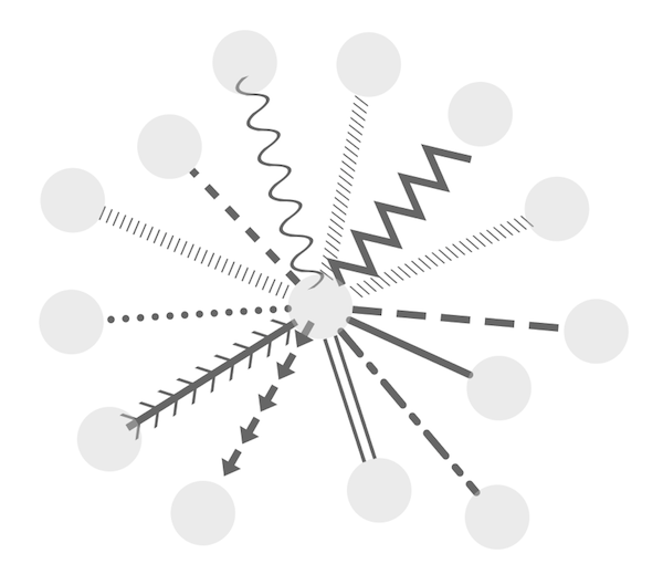
Use specific line types to indicate different types of interactions.
Control edge transparency (opacity) using edge weights.
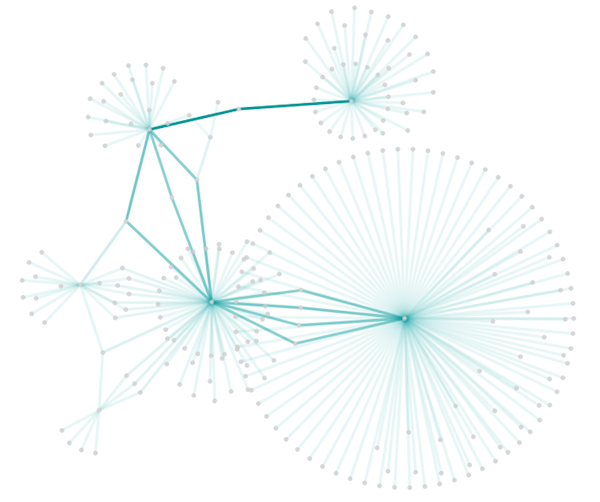
Control multiple edge properties using edge score.
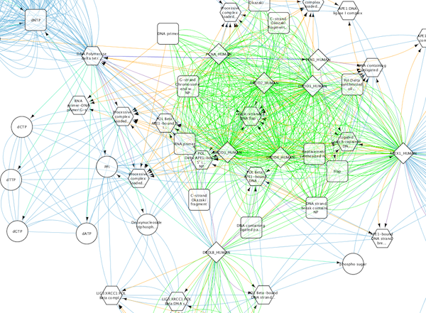
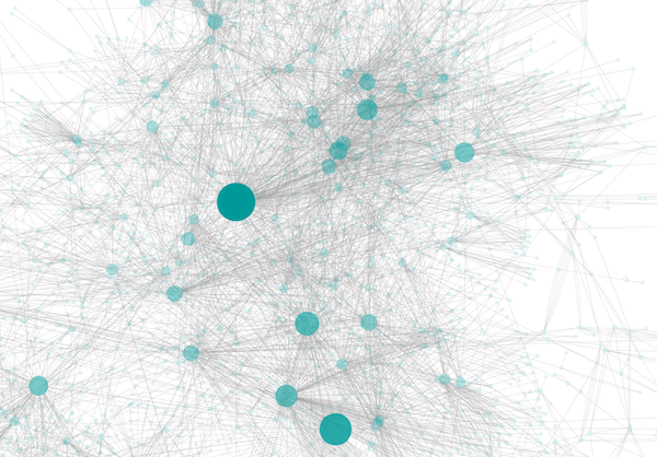
Browse extremely-dense networks by controlling the opacity of nodes.
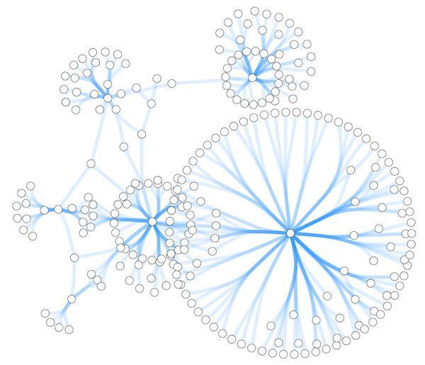
Show highly-connected region by edge bundling and opacity.
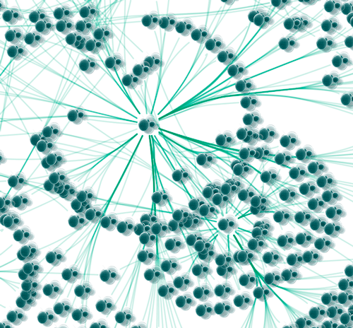
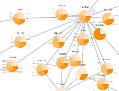
Add photo/image/graphics on top of nodes.
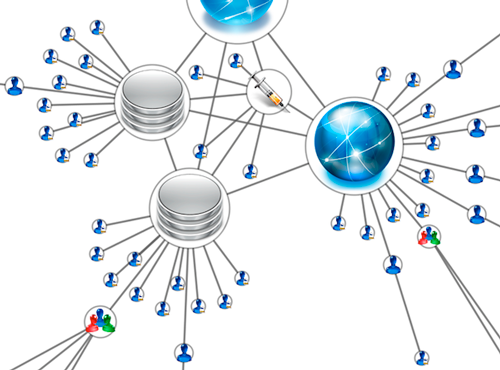
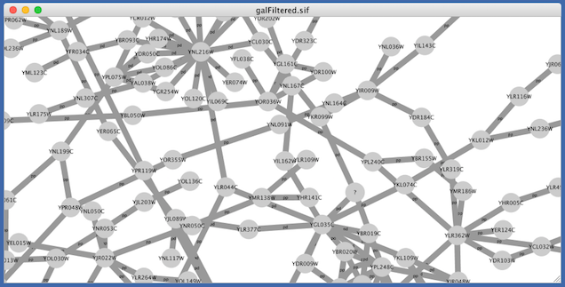
Cytoscape 3 has several sample styles. Below are a few examples of these applied to the galFiltered.sif network :
12.2. Introduction to the Style Interface
The Style interface is located under the Style panel of the Control Panel.
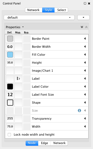
This interface allows you to create/delete/view/switch between different styles using the Current Style options. The panel displays the mapping details for a given style and is used to edit these details as well.
- At the top of the interface, there is a drop-down menu for selecting a pre-defined style. There is also an Options drop-down with options to rename, remove, create and copy a Style, and an option to create a legend for the selected Style.
- The main area of the interface is composed of three tabs, for Node, Edge and Network.
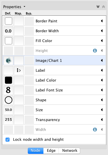
- Each tab contains a list of properties relevant to the current style. At the top of the list a Properties drop-down allows you to add additional properties to the list.
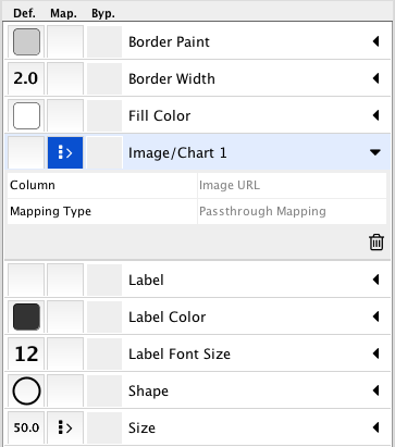
- Each property entry in the list has 3 columns:
- The Default Value shows just that, the default value for the property. Clicking on the Default Value column for any property allows you to change the default value.
- Mapping displays the type of mapping currently in use for the property. Clicking on the Mapping column for any property expands the property entry to show the interface for editing the mapping. Details on the mapping types provided here.
- Bypass displays any style bypass for a selected node or edge. Note that a node/edge or subset of nodes/edges must be selected to activate the Bypass column. Clicking on the Bypass column for selected node(s)/edge(s) allows you to enter a bypass for that property for selected node(s)/edge(s).
The Default Value is used when no mapping is defined for a property, or for nodes/edges not covered by a mapping for a particular property. If a Mapping is defined for a property, this defines the style for all or a subset of nodes/edges, depending on how the mapping is defined. A Bypass on a specific set of nodes/edges will bypass and override both the default value and defined mapping.
12.3. Introduction to Style
The Cytoscape distribution includes several predefined styles to get you started. To examine a few styles, try out the following example:
Step 1. Load some sample data
- Load a sample session file: From the main menu, select File → Open…, and select the file sampleData/galFiltered.cys.
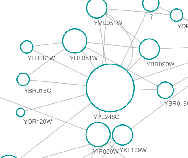
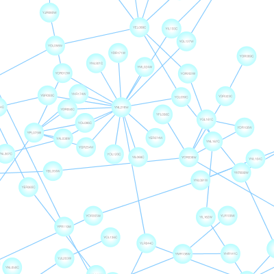
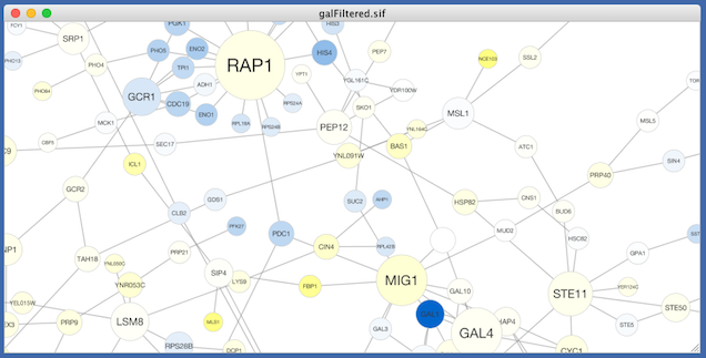
- The session file includes a network, some annotations, and sample styles. By default, the style galFiltered Style is selected. Gene expression values for each node are colored along a color gradient between blue and yellow (where blue represents a low expression ratio and yellow represents a high expression ratio, using thresholds set for the gal1RGexp experiment bundled with Cytoscape in the sampleData/galExpData.csv file). Also, node size is mapped to the degree of the node (number of edges connected to the node) and you can see the hubs of the network as larger nodes. See the sample screenshot below:
Step 2. Switch between different styles
You can change the style by making a selection from the Current Style drop-down list, found at the top of the Style panel.
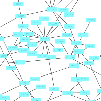
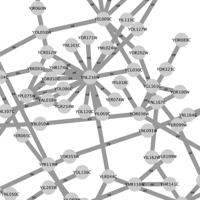
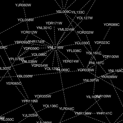
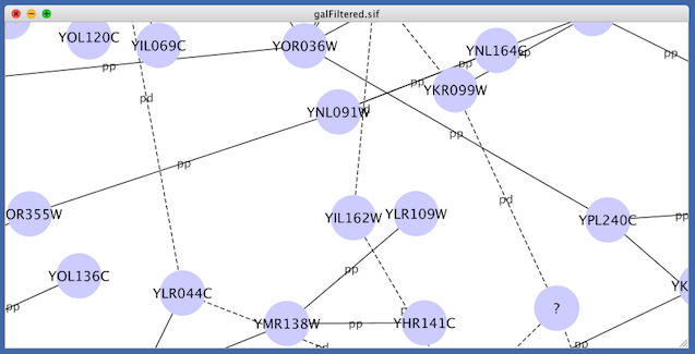
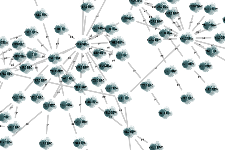
For example, if you select Sample1, a new style will be applied to your network, and you will see a white background and round blue nodes. If you zoom in closer, you can see that protein-DNA interactions (specified with the label “pd”) are drawn with dashed edges, whereas protein-protein interactions (specified with the label “pp”) are drawn with solid edges (see sample screenshot below).
Finally, if you select Solid, you can see the graphics below:
This style does not have mappings except node/edge labels, but you can modify the network graphics by editing the Default Value for any property.
Additional sample styles are available in the sampleStyles.xml file in
the sampleData directory. You can import the sample file from File →
Import → Styles from File….
List of Node, Edge and Network Properties
Cytoscape allows a wide variety of properties to be controlled. These are summarized in the tables below.
| Node Properties | Description |
|---|---|
| Border Line Type | The type of line used for the border of the node. |
| Border Transparency | The opacity of the color of the border of the node. Zero means totally transparent, and 255 means totally opaque. |
| Border Width | The width of the node border. |
| Label | The text used for the node label. |
| Label Font Face | The font used for the node label. |
| Label Font Size | The size of the font used for the node label. |
| Label Position | The position of the node label relative to the node. |
| Label Transparency | The opacity of the node label. Zero means totally transparent, and 255 means totally opaque. |
| Label Width | The maximum width of the node label. If the node label is wider than the specified width, Cytoscape will automatically wrap the label on space characters. Cytoscape will not hyphenate words, meaning that if a single word (i.e. no spaces) is longer than maximum width, the word will be displayed beyond the maximum width. |
| Nested Network Image Visible | A boolean value that indicates whether a nested network should be visualized (assuming a nested network is present for the specified node). |
| Padding (Compound Node) | Internal padding of the compound node (a node that contains other nodes). |
| Paint | The color of the whole node, including its border, label and selected paint. This property can be added to the list from the drop-down menu Properties → Paint → Paint. |
| Border Paint | The color of the border of the node. This property can be added to the list from the drop-down menu Properties → Paint → Border Paint. |
| Image/Chart 1-9 | A user-defined graphic (image, chart or gradient) that is displayed on the node. These properties (maximum of nine) can be added to the list from the drop-down menu Properties → Paint → Custom Paint n → Image/Chart n. |
| Image/Chart Position 1-9 | The position of each graphic (image, chart or gradient). These properties (maximum of nine) can be added to the list from the drop-down menu Properties → Paint → Custom Paint n → Image/Chart Position n. |
| Fill Color | The color of the node. This property can be added to the list from the drop-down menu Properties → Paint → Fill Color. |
| Label Color | The color of the node label. This property can be added to the list from the drop-down menu Properties → Paint → Label Color. |
| Selected Paint | The fill color of the node when selected. This property can be added to the list from the drop-down menu Properties → Paint → Selected Paint. |
| Shape | The shape of the node. |
| Shape (Compound Node) | The shape of the compound node (a node that contains other nodes). |
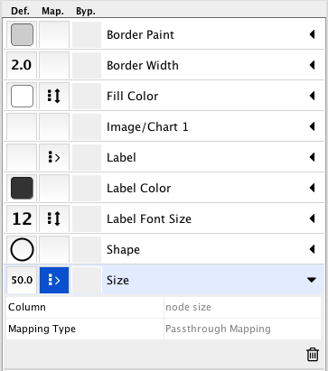
| Size | The size of the node. Width and height will be equal. This property is mutually exclusive of Node Height and Node Width. It can be added to the list from the drop-down menu Properties → Size → Size. |
| Image/Chart Size 1-9 | The size of the related node Image/Chart. It can be added to the list from the drop-down menu Properties → Size → Image/Chart Size n. |
| Height | The height of the node. Height will be independent of width. This property is mutually exclusive of Node Size. It can be added to the list from the drop-down menu Properties → Size → Height. |
| Width | The width of the node. Width will be independent of height. This property is mutually exclusive of Node Size. It can be added to the list from the drop-down menu Properties → Size → Width. |
| Fit Custom Graphics to node | Toggle to fit Image/Chart size to node size. It can be added to the list from the drop-down menu Properties → Size → Fit Custom Graphics to node. |
| Lock node width and height | Toggle to ignore Width and Height, and to use Size for both values. It can be added to the list from the drop-down menu Properties → Size → Lock node width and height. |
| Tooltip | The text of the tooltip that appears when a mouse hovers over the node. |
| Transparency | The opacity of the color of the node. Zero means totally transparent, and 255 means totally opaque. |
| Visible | Hides the node if set to false. By default, this value is set to true. |
| X Location | X location of the node. Default value of this will be ignored. The value will be used only when mapping function is defined. |
| Y Location | Y location of the node. Default value of this will be ignored. The value will be used only when mapping function is defined. |
| Z Location | Z location of the node. Default value of this will be ignored. The value will be used only when mapping function is defined. |
| Edge Properties | Description |
|---|---|
| Bend | The edge bend. Defines how the edge is rendered. Users can add multiple handles to define how to bend the edge line. |
| Curved | If Edge Bend is defined, edges will be rendered as straight or curved lines. If this value is set to true, edges will be drawn as curved lines. |
| Label | The text used for the edge label. |
| Label Font Face | The font used for the edge label. |
| Label Font Size | The size of the font used for the edge label. |
| Label Transparency | The opacity of the color of the edge label. Zero means totally transparent, and 255 means totally opaque. |
| Line Type | The type of stoke used to render the line (solid, dashed, etc.) |
| Paint | The color of the whole edge (including the stroke and arrows) when it is selected or unselected. This property can be added to the list from the drop-down menu Properties → Paint → Paint. |
| Color (Selected) | The color of the whole edge (stroke and arrows) when selected. This property can be added to the list from the drop-down menu Properties → Paint → Color (Selected) → Color (Selected). |
| Source Arrow Selected Paint | The selected color of the arrow on the source node end of the edge. It can be added to the list from the drop-down menu Properties → Paint → Color (Selected) → Source Arrow Selected Paint. |
| Stroke Color (Selected) | The color of the edge line when selected. It can be added to the list from the drop-down menu Properties → Paint → Color (Selected) → Stroke Color (Selected). |
| Target Arrow Selected Paint | The selected color of the arrow on the target node end of the edge. It can be found in the drop-down menu Properties → Paint → Color (Selected) → Target Arrow Selected Paint. |
| Color (Unselected) | The color of the whole edge (stroke and arrows) when it is not selected. It can be found in the drop-down menu Properties → Paint → Color (Unselected) → Color (Unselected). |
| Source Arrow Unselected Paint | The color of the arrow on the source node end of the edge. It can be found in the drop-down menu Properties → Paint → Color (Unselected) → Source Arrow Unselected Paint. |
| Stroke Color (Unselected) | The color of the edge line. It can be found in the drop-down menu Properties → Paint → Color (Unselected) → Stroke Color (Unselected). |
| Target Arrow Unselected Paint | The color of the arrow on the target node end of the edge. It can be found in the drop-down menu Properties → Paint → Color (Unselected) → Target Arrow Unselected Paint. |
| Label Color | The color of the edge label. It can be found in the drop-down menu Properties → Paint → Label Color. |
| Source Arrow Shape | The shape of the arrow on the source node end of the edge. |
| Target Arrow Shape | The shape of the arrow on the target node end of the edge. |
| Tooltip | The text of the tooltip that appears when a mouse hovers over the edge. |
| Transparency | The opacity of the of the edge. Zero means totally transparent, and 255 means totally opaque. |
| Visible | Hides the edge if set to false. By default, this value is set to true. |
| Width | The width of the edge line. |
| Edge color to arrows | If true then Color (Unselected) is used for the whole edge, including its line and arrows. It can be found in the drop-down menu Properties → Paint → Color (Unselected) → Edge color to arrows. |
| NetworkProperties | Description |
|---|---|
| Background Paint | The background color of the network view. |
| Center X Location | The X location of network view center. |
| Center Y Location | The Y location of network view center. |
| Edge Selection | Edges are selectable or not. If this is false, users cannot select edges. |
| Node Selection | Nodes are selectable or not. If this is false, users cannot select nodes. |
| Scale Factor | The zoom level of the network view. |
| Size | The size (width and height) of the network view. It can be found in the drop-down menu Properties → Size → Size. |
| Height | The height of the network view. It can be found in the drop-down menu Properties → Size → Height. |
| Width | The width of the network view. It can be found in the drop-down menu Properties → Size → Width. |
| Title | The title of the network view. |
Available Shapes and Line Styles
| Available Shapes and Line Styles | Sample |
|---|---|
| Node Shapes | 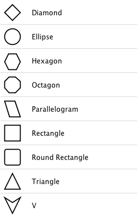 |
| Line Types | 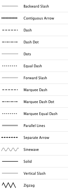 |
| Arrow Shapes | 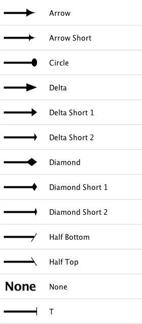 |
How Mappings Work
For each property, you can specify a default value or define a dynamic mapping. Cytoscape currently supports three different types of mappings:
Passthrough Mapping
- The values of network column data are passed directly through to properties. A passthrough mapping is typically used to specify node/edge labels. For example, a passthrough mapping can label all nodes with their common gene names.
Discrete Mapping
- Discrete column data are mapped to discrete properties. For example, a discrete mapping can map different types of molecules to different node shapes, such as rectangles for gene products and ellipses for metabolites.
Continuous Mapping
Continuous data are mapped to properties. Depending on the property, there are three kinds of continuous mapping:
i. Continuous-to-Continuous Mapping: for example, you can map a continuous numerical value to node size.
ii. Color Gradient Mapping: This is a special case of continuous-to-continuous mapping. Continuous numerical values are mapped to a color gradient.
iii. Continuous-to-Discrete Mapping: for example, all values below 0 are mapped to square nodes, and all values above 0 are mapped to circular nodes.
However, note that there is no way to smoothly morph between circular nodes and square nodes.
The table below shows mapping support for each property.
Legend
| Symbol | Description |
|---|---|
| - | Mapping is not supported for the specified property. |
| + | Mapping is fully supported for the specified property. |
| o | Mapping is partially supported for the specified property. Support for "continuous to continuous" mapping is not supported. |
Node Mappings
| Node Property | Passthrough Mapping | Discrete Mapping | Continuous Mapping | |
|---|---|---|---|---|
| Color | Fill Color | + | + | + |
| Transparency | + | + | + | |
| Border Paint | + | + | + | |
| Border Transparency | + | + | + | |
| Label Color | + | + | + | |
| Label Transparency | + | + | + | |
| Numeric | Size/Width/Height | + | + | + |
| Label Font Size | + | + | + | |
| Border Width | + | + | + | |
| Label Width | + | + | + | |
| Padding (Compound Node) | + | + | + | |
| Image/Chart Size | + | + | + | |
| Other | Border Line Type | + | + | o |
| Shape | + | + | o | |
| Shape (Compound Node) | + | + | o | |
| Label | + | + | o | |
| Tooltip | + | + | o | |
| Label Font Face | + | + | o | |
| Label Position | - | + | o | |
| Nested Network Image Visible | + | + | o | |
| Image/Chart | o | + | o | |
| Image/Chart Position | - | + | o | |
Edge Mappings
| Edge Property | Passthrough Mapping | Discrete Mapping | Continuous Mapping | |
|---|---|---|---|---|
| Color | Color | + | + | + |
| Transparency | + | + | + | |
| Target Arrow Color | + | + | + | |
| Source Arrow Color | + | + | + | |
| Label Color | + | + | + | |
| Label Transparency | + | + | + | |
| Numeric | Width | + | + | + |
| Label Font Size | + | + | + | |
| Label Width | + | + | + | |
| Other | Line Type | + | + | o |
| Bend | - | + | o | |
| Curved | + | + | o | |
| Source Arrow Shape | + | + | o | |
| Target Arrow Shape | + | + | o | |
| Label | + | + | o | |
| Tooltip | + | + | o | |
| Label Font Face | - | + | o | |
Text Passthrough Mapping
In Cytoscape 2.8.0 and later versions, the Passthrough Mapping can recognize some text representations of values. This means, if you have a string column named Node Size Values, you can directly map those values as the Node Size by setting “Node Size Values” as controlling column with Node Size “Passthrough Mapping”. The following value types are supported:
- Colors: Standard color names supported by all browsers or RGB representation in hex
- Numerical Values: Automatically mapped to the specified property.
- Images: URL String. If the URL is valid and an actual image data exists there, Cytoscape automatically downloads the image and maps it to the node.
12.4. Images, Charts and Gradients
Cytoscape allows you to set custom graphics to nodes. Using the Style interface, you can map Image/Chart properties to nodes like any other property. Cytoscape provides a set of images and you can also add your own images in the Image Manager, as well as remove or modify existing ones.
Taxonomy Icon (http://biosciencedbc.jp/taxonomy_icon/taxonomy_icon.cgi?lng=en) set used in this section is created by Database Center for Life Science (DBCLS) and is distributed under Creative Commons License (CC BY 2.1.)
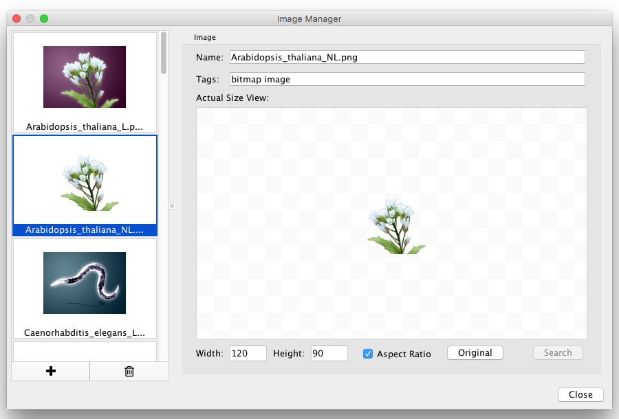
Managing Images
The Image Manager is available under the menu option View → Open Image Manager…:
- You can add images by drag-and-drop of image files and URLs. If you
want to add images from a web browser or local file system, you can
drag images from them and drop those images onto the list of images
on the left.
- Note: When you drag and drop images from web browser, make sure that you are actually dragging the URL for the image. In some cases, images are linked to an HTML page or scripts, and in such cases, this drag and drop feature may not work.
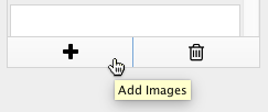
- If you want to add one or more images from a folder, press the + button on the bottom of the Image Manager window and then select the images you want to add.
- To remove images from the current session’s image library, simply select one or more images from the list and press the Remove Selected Images button (trash icon).
- Images can be resized by defining specific Width and Height values. If the Aspect Ratio box is checked, the width-height ratio is always synchronized. You can resize the image to the original size by pressing the Original button.
Using Graphics in Styles
Node graphics are used and defined like any other property, through the Style interface. There are nine Image/Chart properties.
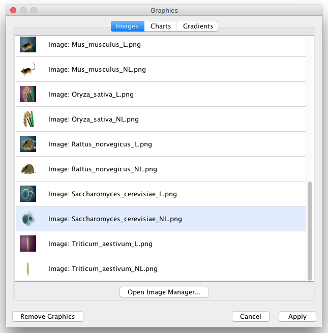
- Cytoscape provides three kinds of graphics (selectable via tabs on
the Graphics dialog):
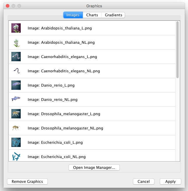
- Images: You can select one of the provided images or add your own (click the Open Image Manager… button to add more images to the list).
- Charts: The following chart types are available:
 Bar ,
Bar ,
 Box,
Box,
 Heat Map,
 Line,
Line,
 Pie,
Pie,
 Ring.
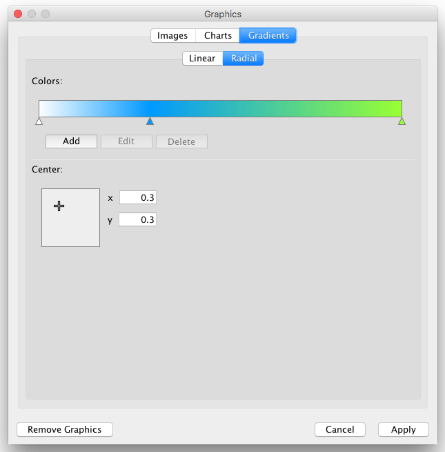
Ring. - Gradients: You can also set Linear and Radial gradients to nodes.
- To add a graphic, first add one Image/Chart property to the
properties list in the Style interface (on the Node tab,
select Properties → Paint → Custom Paint n → Image/Chart n).
Next, click the Default Value column of the Image/Chart
property to bring up the Graphics dialog. Select an image, a
chart or a gradient and then click Apply.
- By default, graphics are automatically resized to be consistent with the Node Size property.
- To remove an image, chart or gradient, click the Remove Graphics button on the Graphics dialog.
Graphics Positions
Each Image/Chart property is associated with a position. You can edit its position by using the UI available in the Default Value column for the Image/Chart Position property that has the same number. For instance, the Image/Chart Position 2 value modifies the position of Image/Chart 2.
- Note: Setting graphics positions for Linear or Radial gradients has no effect, as they are always centered on the node.
Z-Ordering
The number that appears with the Image/Chart property represents an ordering of layers. Basic node color and shape are always rendered first, then node Image/Chart 1, 2, …, through 9.
Saving and Loading Images
In general, saving and loading images is automatic. When you quit Cytoscape, all of the images in the Image Manager will be saved automatically. There are two types of saving:
- To a session file
- When you save the current session to a file, the images used in the current styles will be saved to that file. For example, if you have a style with a discrete mapping for Image/Chart 1, all images used in the style will be saved to the session file. Other images will not be saved in your session file. This is because your image library can be huge when you add thousands of images to the Image Manager and it takes a very long time to save and load the session file.
- Automatic saving to
CytoscapeConfiguration/images3directory- When you select File → Quit (Windows and Linux) or
Cytoscape → Quit Cytoscape (Mac OS X), all of the images in
the Image Manager will be saved automatically to your Cytoscape
settings directory. Usually, they are saved in
YOUR_HOME_DIRECTORY/CytoscapeConfiguration/images3.
- When you select File → Quit (Windows and Linux) or
Cytoscape → Quit Cytoscape (Mac OS X), all of the images in
the Image Manager will be saved automatically to your Cytoscape
settings directory. Usually, they are saved in
In any case, images will be saved automatically to your system or session and will be restored when you restart Cytoscape or load a session.
12.5. Styles Tutorials
The following tutorials demonstrate some of the basic Style features. Each tutorial is independent of the others.
Tutorial 1: Creating a Basic Style and Setting Default Values
The goal of this tutorial is to learn how to create a new Style and set some default values.
Load a sample network: From the main menu, select File → Import → Network from File…, and select
sampleData/galFiltered.sif.Create some node/edge statistics: The Network Analyzer calculates some basic statistics for nodes and edges. From the main menu, select Tools → Network Analyzer → Network Analysis → Analyze Network, and click OK. Once the result is displayed, simply close the window. All statistics are stored as regular table data.
Select the Style panel in the Control Panel.
Create a new style: Click the Options
 drop-down, and select Create New Style. Enter a name for your
new style when prompted.
drop-down, and select Create New Style. Enter a name for your
new style when prompted.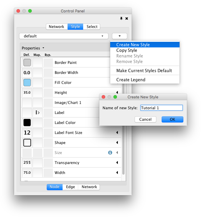
Since no mappings are set up yet, only default values are defined for some of the properties. From this panel, you can create node/edge mappings for all properties.
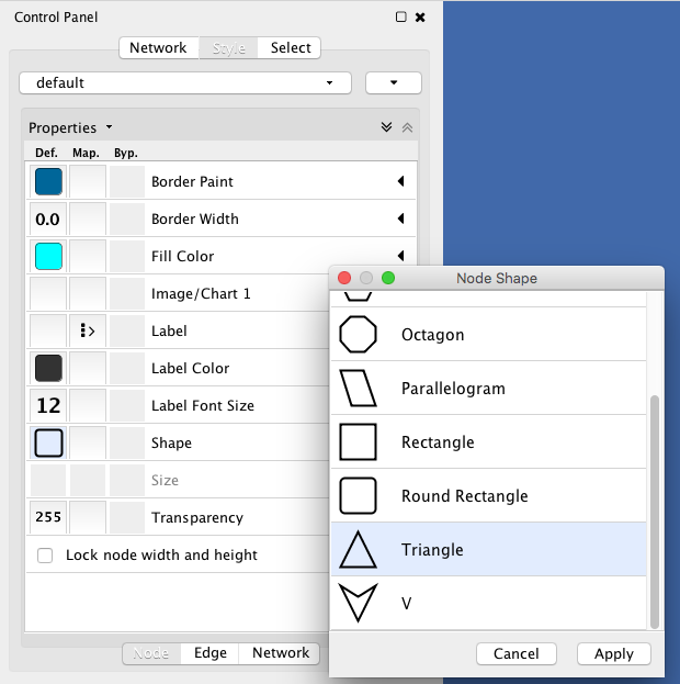
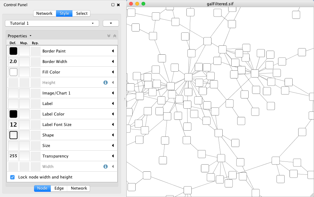
Change the default node color and shape: To set the default node shape to triangles, click the Default Value column for the Shape property. A list of available node shapes will be shown. Select the Triangle item and click the Apply button. You can edit other default values in the same way. In the example shown below, the node shape is set to Round Rectangle, while Fill Color is set to white. The new Style is automatically applied to the current network, as shown below.
Tutorial 2: Creating a New Style with a Discrete Mapping
Now you have a network with a new Style. The following section demonstrates how to create a new style that has a discrete mapping. The goal is to draw protein-DNA interactions as dashed lines, and protein-protein interactions as solid lines.
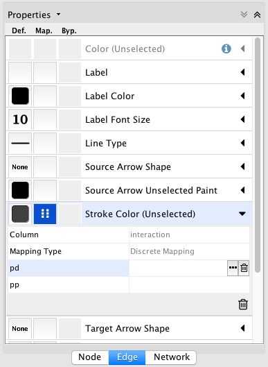
Find the property: In the Edge tab of the Style panel, find the Stroke Color (Unselected) property. If it is not already visible in the properties sheet, add it by selecting the drop-down item Properties → Paint → Color (Unselected) → Stroke Color (Unselected).
Choose a data column to map to: Expand the entry for Stroke Color (Unselected) by clicking the arrow icon on the right. Click the Column entry and select “interaction” from the drop-down list that appears.
Set the mapping type: Under Mapping Type, select “Discrete Mapping”. All available column values for “interaction” will be displayed, as shown below.
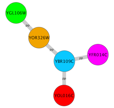
Set the mapped values: Click the empty cell next to “pd” (protein-DNA interactions). On the right side of the cell, click on the … button that appears. A popup window will appear; select green or similar, and the change will immediately appear on the network window.
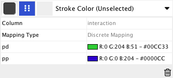
Repeat step 4 for “pp” (protein-protein interactions), but select a darker color. Then repeat steps 3 through 4 for the Line Type property, by selecting the correct line style (“Dash” or “Solid”) from the list.
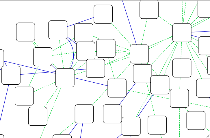
Now your network should show “pd” interactions as dashed green lines and “pp” interactions as solid lines. A sample screenshot is provided below.
Tutorial 3: Creating a New Style with a Continuous Mapping
At this point, you have a network with some edge mappings. Next, let’s create mappings for nodes. The following section demonstrates how to create a new style using a continuous mapping. The goal is to superimpose node statistics (in this example, node degree) onto a network and display it along a color gradient.
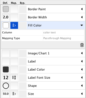
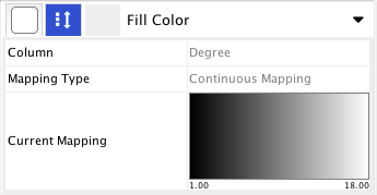
Find the property: In the Node tab of the Style panel, find the Fill Color property. If it is not already visible in the properties sheet, add it by selecting the drop-down item Properties → Paint → Fill Color.
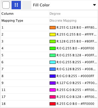
Set the node table column: Expand the entry for Fill Color by clicking the arrow icon on the right. Click the Column entry and select “Degree” from the drop-down list that appears.
Set the mapping type: Set the “Continuous Mapping” option as the Mapping Type. This automatically creates a default mapping.
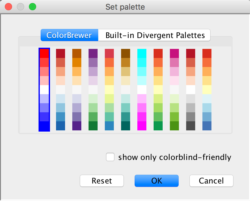
Define a color palette. We encourage you to choose palette from the existing ones provided, but you can also choose the color states yourself and provide any number of intermediate colors. Both methods are described here.
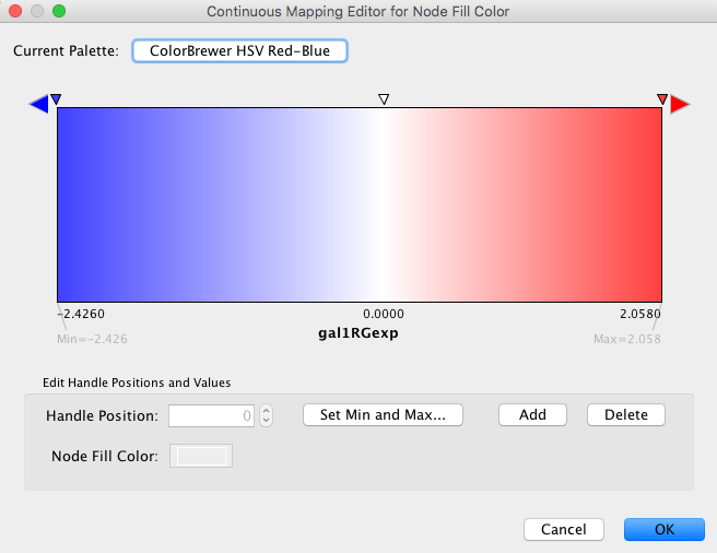
4A. Choose a predefined palette from the Palette picker. These come from published recommendations for choosing colors in scientific and cartographic applications, such as BrewerColors. Click the Current Palette button in the top left of the Continuous Mapping Editor to choose from a set of palettes. Below shows the Set Palette dialog to choose a full palette.
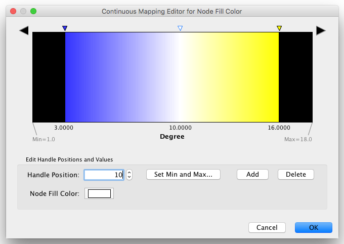
4B. Define the points where colors will change: Double-click on the black-and-white gradient rectangle next to Current Mapping to open the Continuous Mapping Editor. Note the two smaller triangles at the top of the gradient.
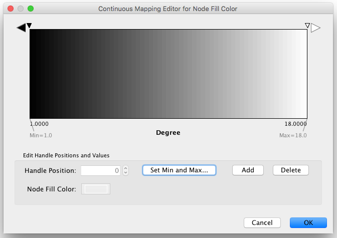
Define the colors between points: Double-click on the larger leftmost triangle (facing left) and a color palette will appear. Set the color white and repeat for the smaller left-side triangle. For the triangle on the right, set the color green and then choose the same color for the smaller right-side triangle.
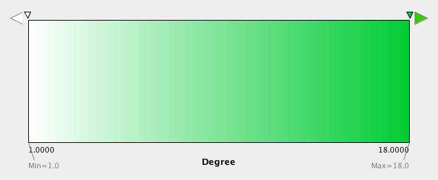
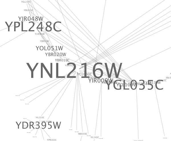
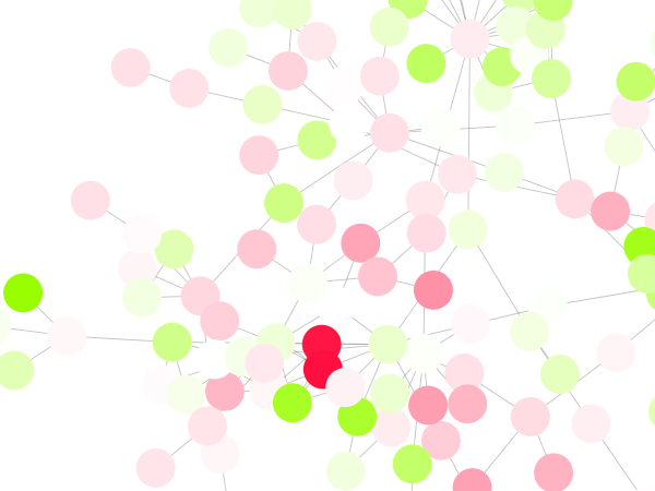
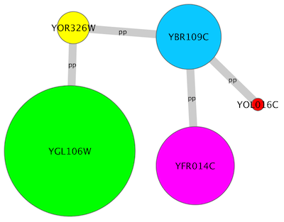
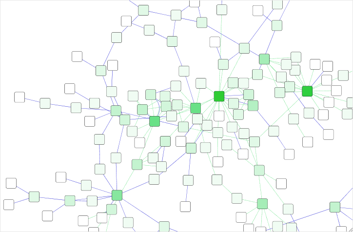
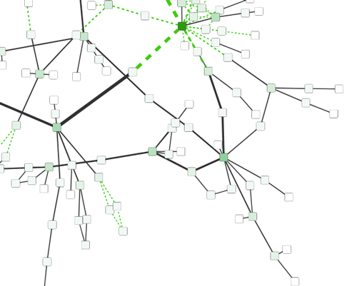
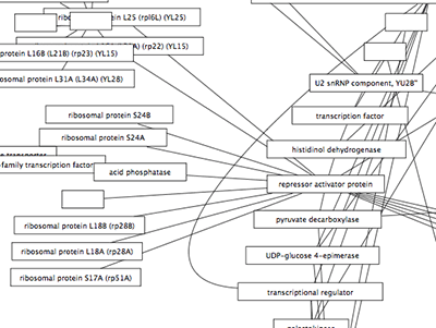
The color gradients will immediately appear on the network. All nodes with degree 1 will be set to white, and all values between 1 and 18 will be painted with a white/green color gradient (see the sample screenshot below).
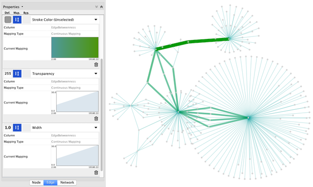
Repeat for other properties: You can create more continuous mappings for other numeric table data. For example, edge data table column “EdgeBetweenness” is a number, so you can use it for continuous mapping. The following is an example visualization which mapps Edge Width to “EdgeBetweenness”.
Tutorial 4: Setting Automatic Values to a Discrete Mapping
The goal of this section is to learn how to generate automatic values for discrete mappings.
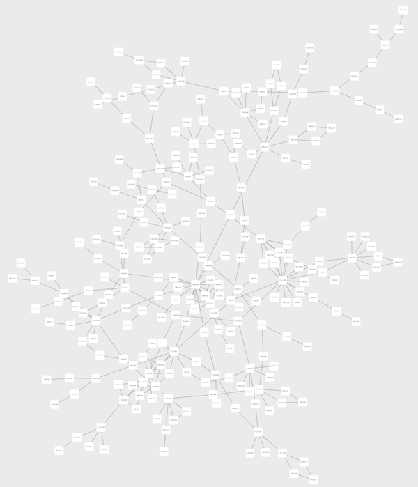
Switch the Current Style to Minimal. Now your network looks like the following:
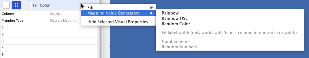
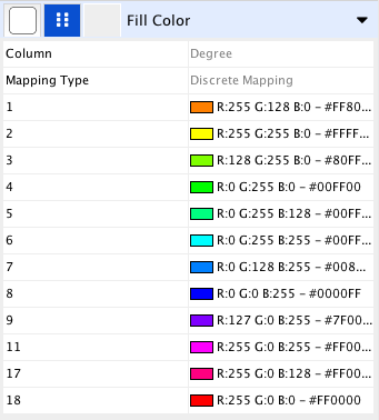
Create a discrete mapping for Fill Color. Select “AverageShortestPathLength” (generated by the Network Analyzer) as the controlling property.
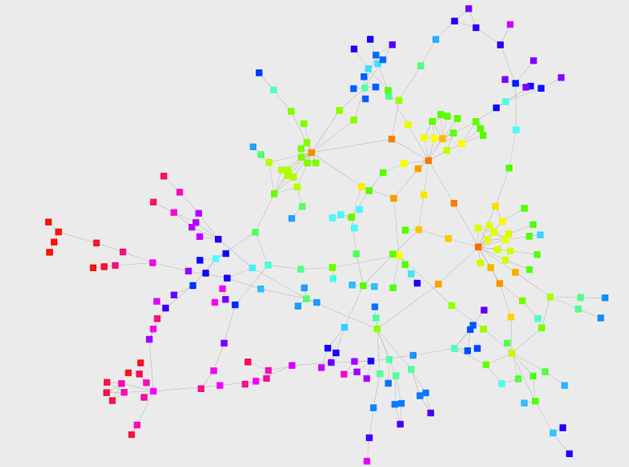
Right-click the Fill Color cell, then select Mapping Value Generators → Rainbow. Cytoscape will automatically generate different colors for all the property values as shown below:
Create a discrete mapping for Label Font Size. Select “AverageShortestPathLength” as controlling property (Column field).
Right-click the Label Font Size cell, then select Mapping Value Generators → Number Series. Type 3 for the first value and click OK. Enter 3 for increment.
Apply Layout → yFiles Organic Layout. The final view is shown below:
This mapping generator utility is useful for categorical data. The following example shows a discrete mapping that maps the species column to node color.
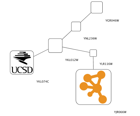
Tutorial 5: Using Images in Styles
This tutorial is a quick introduction to the node image feature. You can assign up to nine images per node as a part of a Style.
In this first example, we will use the presets that Cytoscape 3 has. In general, you can use any type of bitmap graphics. User images should be added to the Image Manager before using them in a Style.
If you are continuing from the previous tutorials, skip to the next step. Otherwise, load a network and run the Network Analyzer (Tools → Network Analyzer → Network Analysis → Analyze Network…). This creates several new table columns (statistics for nodes and edges).
Click the Style panel in the Control Panel, and select the Solid style.
If the property Image/Chart 1 is not in the properties sheet yet, add it from the drop-down Properties → Paint → Custom Paint 1 → Image/Chart 1.
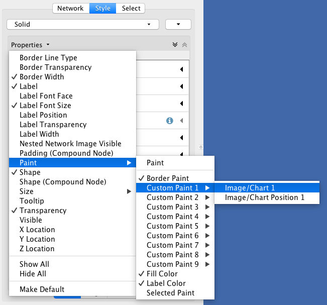
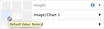
Click the Default Value cell of the Image/Chart 1 entry in order to open the Graphics dialog.
Select any of the images from the list and click Apply.
Click the Default Value cell of node Transparency and set the value to zero.
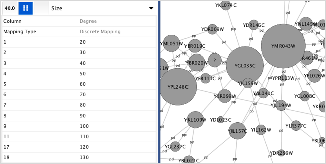
Set the Default Value of node Size to 80.
Set the Default Value of node Label Font Size to 10, to increase readability.
Also change the edge Width to 6. Now your network looks like the following:
Open the Image Manager under View → Open Image Manager…. Drag and Drop this
 icon to the image list which automatically adds it to the manager.
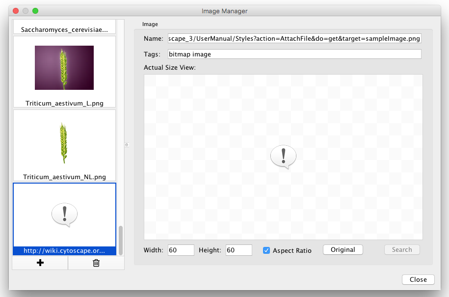
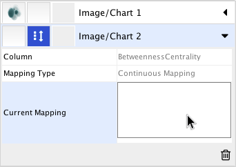
Create a Continuous Mapping for Image/Chart 2 and select “BetweennessCentrality” as its controlling property. Double-click the Current Mapping value cell to open the Continuos Mapping Editor.
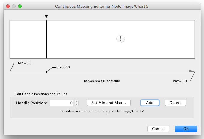
In the Continuos Mapping Editor, add a handle position by clicking in the Add button, and move the handle to 0.2. Double-click the region over 0.2 and set the new icon you have just added in the last step.
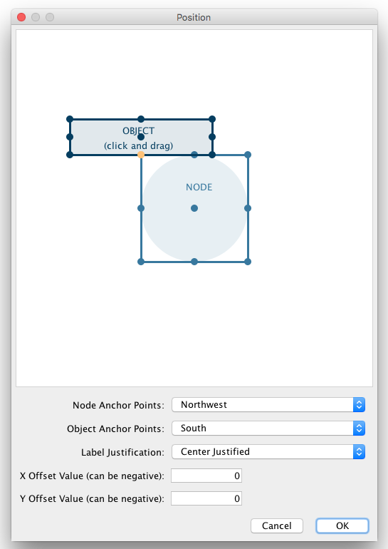
Add the property Image/Chart Position 2 from the drop-down option Properties → Paint → Custom Paint 2 → Image/Chart Position 2. Click its Default Value cell to move the position of the graphics to upper left.
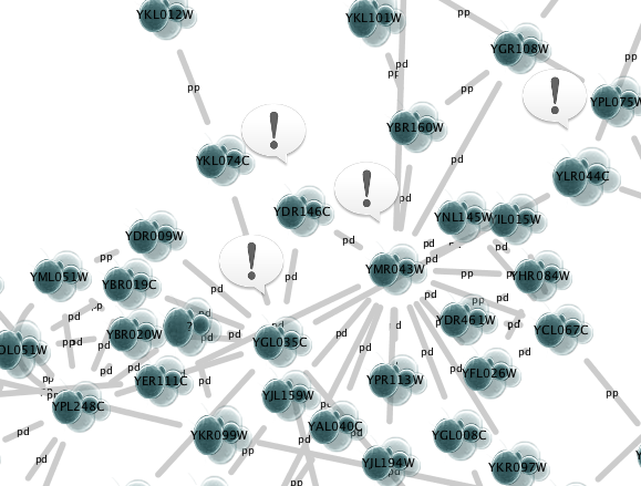
Now the important nodes in the network (nodes with high betweenness centrality) are annotated with the icon:
Tutorial 6: Creating Node Charts
The goal of this tutorial is to learn how to create and customize node charts from data stored in the Node tables.
Start a new session and load a sample network. From the main menu, select File → Import → Network from File…, and select
sampleData/galFiltered.sif.Create some node/edge statistics using the Network Analyzer. Network Analyzer calculates some basic statistics for nodes and edges. From the main menu, select Tools → Network Analyzer → Network Analysis → Analyze Network…, and click OK. Once the result is displayed, simply close the window. All statistics are stored as regular table data.
Select the Style panel in the Control Panel.
Create a new style: Click the Options
drop-down, and select Create New Style. Enter a name for your
new style when prompted.If the property Image/Chart 1 is not in the properties sheet yet, add it from the drop-down Properties → Paint → Custom Paint 1 → Image/Chart 1.
Click the Default Value cell of the Image/Chart 1 entry in order to open the Graphics dialog.
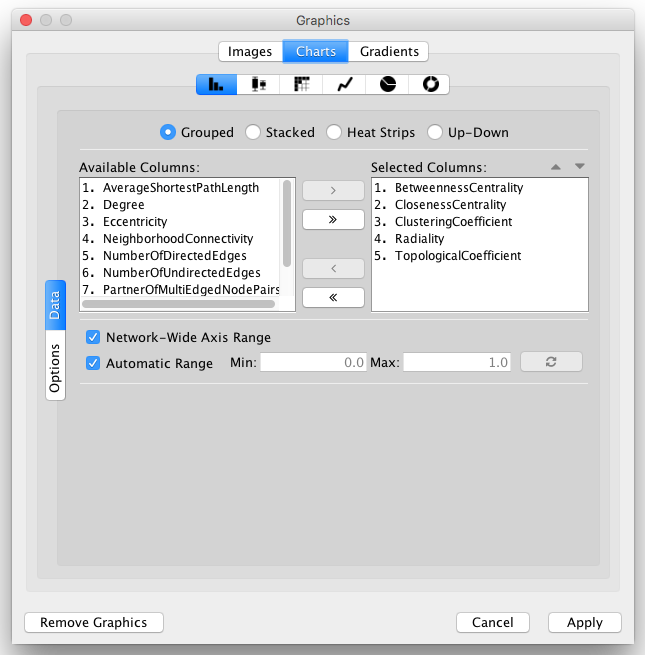
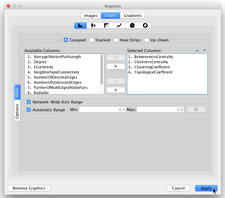
Click the Charts tab and make sure the Bar Chart option is selected.
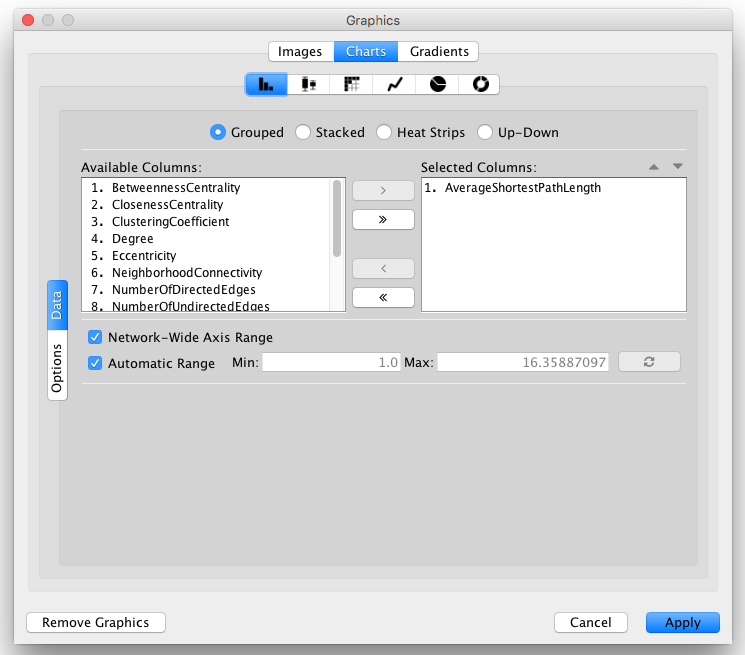
Select data columns: Now you have to choose the columns in the Node table that contains the data you want to be displayed as charts. The Available Columns list displays all node columns that can be used as chart data (i.e. single or list columns of numerical types).
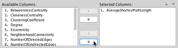
First click the Remove All button to remove the current selected columns (by default, Cytoscape selects the first column in the Available Columns list).
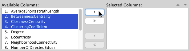
Now select all centrality and coefficient columns from Available Columns list and click the Add Selected button.
Click the Apply button to create bar charts with the selected data columns and default options.
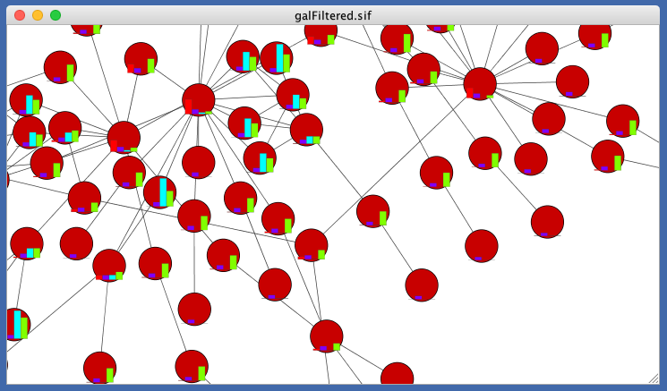
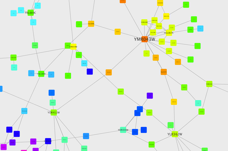
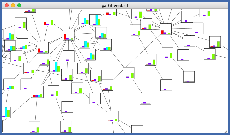
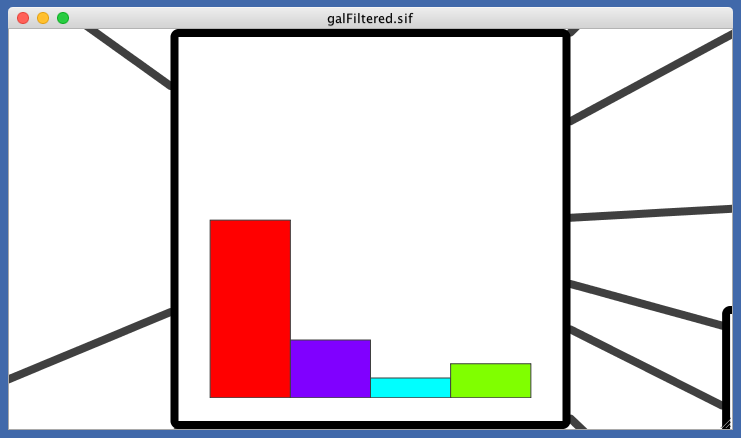
The network view doesn’t look so good yet, so let’s make a few changes to its Style before we continue. In the example shown below, the node Shape is set to Rectangle, while the node Fill Color is set to white.
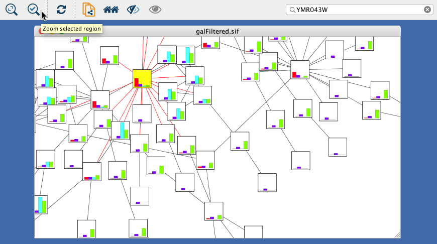
Focus on one node to see the chart details. For example search for and then focus on node “YMR043W”.
Change other chart options: Click the Default Value cell of the Image/Chart 1 property again in order to open the Graphics dialog, and then select the Options tab on the Bar Chart editor.
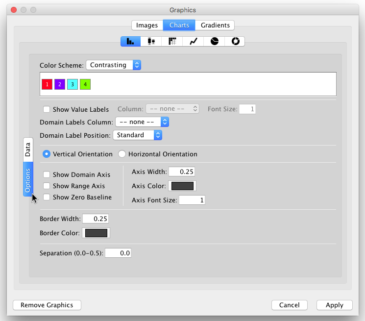
On this panel, you can:
- Choose another Color Scheme or set all the colors individually (just click on each color).
- Show/Hide Value and Domain Labels and also set the Domain Label Position.
- Change the chart Orientation.
- Show/Hide Axes.
- Change the line width and color for axes and bars.
- Increase or reduce the separation between bars (up to 50% of the total chart width).
- Note: Other charts provide different options.
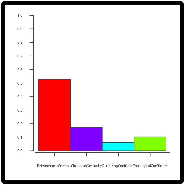
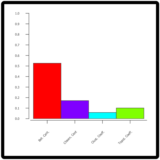
Check both Show Domain Axis and Show Range Axis and apply the graphics again. Now the node chart should look like this:
The default domain labels are not very useful, so let’s set better labels:
- On the Node Table (Table Panel), create a new List Column of type String and name it “domain_labels”.
- Edit any of the cells of the created column (double-click it)
and type
["Bet. Cent.","Closen. Cent","Clust. Coeff.","Topol. Coeff."]. - Right-click the same cell and select the option Apply to entire column.
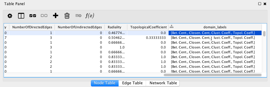
- Open the chart editor again and select the Options panel.
- Select “domain_labels” on the Domain Labels Column drop-down button.
- Select “Up 45^o^” on the Domain Labels Position drop-down button. The labels should look like this now:
12.6. Advanced Topics
Discrete Mappings
Several utility functions are available for Discrete Mappings. You can use these functions by right-clicking on any property entry (shown below).
Automatic Value Generators
Mapping Value Generators - Functions in this menu category are value generators for discrete mappings. Users can set values for discrete mappings automatically by selecting these functions.
Rainbow and Rainbow OSC - These functions try to assign as diverse a set of colors as possible for each data value.
Random Numbers and Random Colors - Randomized numbers and colors.
Number Series - Set a series of numbers to the specified mapping. Requires a starting number and increment.
Fit label width - This function is only for node Width and Size. When a discrete mapping for node Width or Size is available, you can fit the size of each node to its label automatically by selecting this function. See the example below:
Edit Selected Values at Once
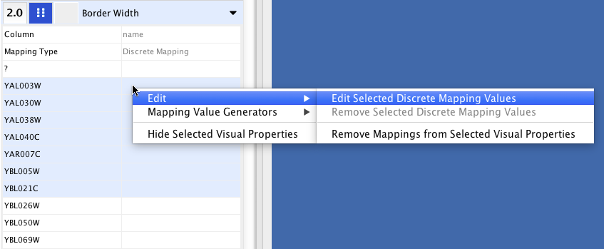
You can set multiple values at once. First, you need to select discrete mapping rows in which you want to change values then right-click and select Edit → Edit Selected Discrete Mapping Values. A dialog pops up and you can enter the new value for the selected rows.
Working with Continuous Mapping Editors
There are three kinds of Continuous Mapping Editors. Each of them are associated with a specific property type:
| Editor Type | Supported Data Type | Properties |
|---|---|---|
| Color Gradient Editor | Color | node/edge/border/label colors |
| Continuous-Continuous Editor | Numbers | size/width/transparency |
| Continuous-Discrete Editor | All others | font/shape/text/graphics/position/etc. |
Range Settings Panel
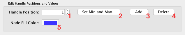
Each continuous mapping editor has a range settings section (labelled Edit Handle Positions and Values) with the following fields and buttons.
- Handle Position - This box displays the current value for the selected slider handle. You can also directly type the value in this box to move the slider to an exact location.
- Set Min and Max… - Click this button to set the overall range of this editor. The first time you open the editor, the Min and Max values are set by the range of the data column you selected (i.e. the minimum and maximum values of the mapped column). In the pop-up dialog you can manually enter the Min and Max values, or they can be set to the current minimum and maximum values of the data column by clicking the Reset button.
- Add - Adds a new handle to the editor.
- Delete - Deletes the selected handle from the slider widget.
- Handle Value (e.g. Node Fill Color) - Click this button to edit the value (e.g. a color) assigned to the selected handle.
Gradient Editor
The Gradient Editor is an editor for creating continuous mappings for colors. To change the color of each region, just double-click the handles (small triangles on the top). A Color gradient will be created only when the editor has two or more handles (see the example below).
| 1 handle (no gradient) | 2 handles |
|---|---|
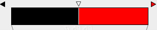 | 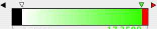 |
Continuous-Continuous Editor
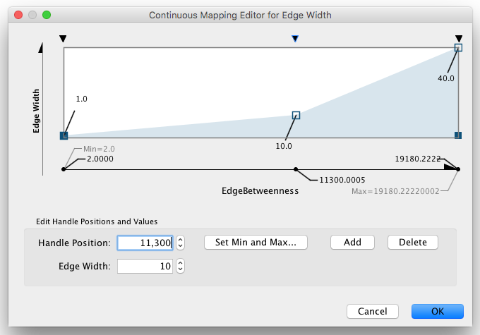
The Continuous-Continuous Editor is for creating mappings between numerical data and numerical properties (e.g. size, transparency). To change the value assigned on the Y-axis (the property shown in the example above is edge Width), drag the small squares or double-click them to directly type an exact value.
Continuous-Discrete Editor
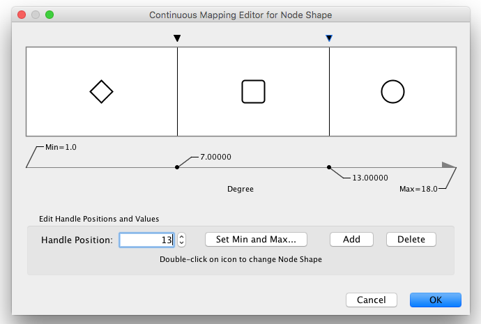
The Continuous-Discrete Editor is used to create mappings from numerical column values to discrete properties, such as fonts, shapes, or line styles. To edit a value for a specific region, double-click the icon on the track.
12.7. Managing Styles
All Cytoscape Style settings are initially loaded from a default file
that cannot be altered by users. When users make changes to the
properties, a session_syle.xml file is saved in the session file. This
means that if you save your session, you will not lose your properties.
No other style files are saved during normal operation.
Saving Styles
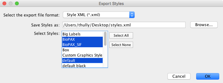
Styles are automatically saved with the session they were created in. Before Cytoscape exits, you will be prompted to make sure you save the session before quitting. It is also possible to save your styles in a file separate from the session file. To do this, navigate to the menu option File → Export → Styles…, and save the selected styles to a file. This feature can be used to share styles with other users.
You can also change the default list of styles for all future sessions
of Cytoscape. To do this, click the Options
drop-down in the Style section, and select Make Current Styles
Default. This will save the current styles as a default_vizmap.xml
file to your CytoscapeConfiguration directory (found in your home
directory). These styles will then be loaded each time Cytoscape is
started.
Style File Formats
The Cytoscape-native Style format is Style XML. If you want to share Style files with other Cytoscape users, you need to export them to this format.
From version 3.1.0 on, Cytoscape can also export Cytoscape.js compatible JSON file. Since Cytoscape.js is an independent JavaScript library, and there are some differences between Cytoscape and Cytoscape.js, not all properties are mapped to JSON. The following properties are not supported by the exporter:
- Custom Graphics and their locations
- Edge Bends
- Nested Networks
- Network Background (Note: This can be set manually as standard CSS in Cytoscape.js)
The Continuous-Discrete Editor is used to create mappings from numerical data values to discrete properties, such as fonts, shapes, or line styles. To edit a value for a specific region, double-click on the icon on the track.
Importing Styles
To import existing styles, navigate to the menu option File → Import →
Styles from File… and select a styles.xml (Cytoscape 3 format) file.
Imported properties will supplement existing properties or override
existing ones if the properties have the same name. You can also specify
a style file using the -V command line option. Properties loaded from
the command line will override any default properties. Note that legacy
menu, but not by command line.